Anomaly Detection
The objective of an Anomaly Detection Task is to learn what is normal in a dataset, and create an alert if the new values deviate from the normal dataset, by user specified threshold. Learning is done during the Training phase and alert creation is done during the Inference phase. The dataset for both Training and Inference phases is provided by running FortiSIEM reports.
- Anomaly Detection Algorithms for Local Mode
- Running Anomaly Detection Local Mode
- Anomaly Detection Algorithms for AWS Mode
- Running Anomaly Detection AWS Mode
Anomaly Detection Algorithms for Local Mode
In this mode, the following algorithms can run locally within the FortiSIEM Supervisor/Worker cluster.
Bipartite Graph Edge Anomaly Detection Algorithm
This is a proprietary machine learning algorithm that tries to detection login anomalies by learning the login patterns and forming dynamic user peer groups. A bipartite graph is a graph where the sets of nodes can be split into two disjoint sets such that there are no edges between the nodes within the same set. An example is Users and Workstations where the edge between a user and a Workstation represents a login, and the edge weight can be the number of logins. The anomaly detection algorithm works as follows. During the training phase, a similarity score between a user/workstation and another user/workstation is calculated. The principle behind similarity score calculation is as follows:
- The similarity score between a user and a workstation is high if the user accesses that workstation.
- The similarity score between two users is high if they access similar workstations.
- The similarity score between two workstations is high if they are accessed by a common set of users.
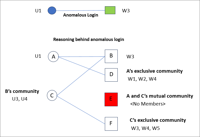
During testing and inference phases, a login from user (A) to a workstation (B) is considered anomalous if the similarity score between user A and the other users that typically access workstation B is lower than a user defined threshold. More specifically:
- C: The set of users that access workstation B during training phase. This is B’s community.
- E: The set of workstations that are accessed by both A and C during training phase. This is A and C’s mutual community.
- D: The set of workstations that are accessed by only A during training phase. This is A’s exclusive community.
- F: The set of workstations that are accessed by only C during training phase. This is C’s exclusive community.
For an anomaly to occur, the set of workstations E should be far fewer compared to set of Workstations D (A’s exclusive community) and F (C’s exclusive community). If this is not the case, then consider reducing the anomaly threshold.
As an example, consider the following login scenario between users U1, U2, U3, U4 and Workstations W1, W2, W3, W4. The login is modeled as a weighted Bipartite graph as shown below.
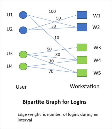
A login from user U1 to Workstation W3 is considered an anomaly because user U1 and W3’s user community (namely U3 and U4) do not access common workstations.
There are 3 parameters for this algorithm:
- Threshold : Scores lower than this threshold is considered anomalous.
- Max node degree: Nodes with degree higher than this value will be ignored. In the User and Workstation case.
- Users that access more than max node degree workstations will be ignored.
- Workstations that are accessed by more than max node degree users will be ignored.
- Convergence bound: Bipartite Edge Anomaly Algorithm stops if the change in reward matrix is lower than this value. This is an internal parameter.
The following groups of users/workstations are eliminated during testing and inference phases, and they do not raise incidents:
- Users that access many workstations (e.g., Domain Admins in Microsoft Active Directory environments).
- Workstations that are accessed by many users (e.g., Microsoft Active Directory)
- Users or Workstations that were never seen during the training phase and hence not part of the model. A periodic retraining would resolve this issue.
Elliptic Envelope Algorithm
An unsupervised anomaly detection algorithm which constructs an ellipsoid around the center of the data points. If a data point falls outside the Ellipsoid, then it is considered as an anomaly. This is suitable for Gaussian distributed data. The parameters for this algorithm are described here: https://scikit-learn.org/stable/modules/generated/sklearn.covariance.EllipticEnvelope.html
Isolation Forest Algorithm
An unsupervised anomaly detection algorithm that builds a random tree by randomly selecting a feature and then randomly selecting a split value between the maximum and minimum values of that feature. If a data point has a small path from the root of the tree, then it is considered as an anomaly. The parameters for this algorithm are described here: https://scikit-learn.org/stable/modules/generated/sklearn.ensemble.IsolationForest.html
Local Outlier Factor Algorithm
An unsupervised anomaly detection algorithm which computes the local density deviation of a data point with respect to its neighbors. If a data point has substantially lower density than their neighbors, then it is considered as an anomaly. The parameters for this algorithm are described here: https://scikit-learn.org/stable/modules/generated/sklearn.neighbors.LocalOutlierFactor.html
Statistical Deviation Algorithm
An unsupervised anomaly detection algorithm based on mean, median, standard deviation and absolute median deviation. A data point is considered an anomaly if the difference between current value and sample mean (or sample median) in a Window is more than a user specified multiplier times the standard deviation (respectively absolute median deviation) over the same window. This is a generalization of the Z-score based methods. The parameters for this algorithm are:
- Mode: Std (meaning Standard Deviation) or Median Absolute (meaning MedAbs)
- Multiplier: It will be used to calculate the lower/upper bound
- Window: Length of sliding window for calculating mean, median and standard deviation
Specially,
- For Mode=Std: a data point is anomalous if the absolute difference between current value and sample mean in the Window is more than Multiplier times the Standard Deviation over the same Window
- For Mode= MedAbs: a data point is anomalous if the absolute difference between current value and sample median in the Window is more than Multiplier times the Median Deviation over the same Window
Running Anomaly Detection Local Mode
Step 1: Design
First identify the following items:
- Fields to Analyze – these fields will be considered for anomaly detection. Currently each field must be a numerical field.
- Time field – this field is required for Statistical Deviation algorithms. It is optional for other algorithms.
- A FortiSIEM Report to get this data.
Requirements
- Report must contain one or more numerical fields to use for anomaly detection. To provide several samples, you can provide a time field. This is optional.
- Each field must be present in the report result; else the whole row will be ignored by the Machine Learning algorithm.
- There can be columns other than the Fields to Analyze in the report and they will be ignored by the machine learning algorithm. However, it is recommended to remove unnecessary columns from the dataset to reduce the size of the dataset exchanged between App Server and phAnomaly modules, during Training and Inference.
Go to Analytics > Search and run various reports. Once you have the right report, save it in Resources > Machine Learning.
Step 2: Prepare Data
Prepare the data for training.
- Go to Analytics > Machine Learning, and click the Import Machine Learning Jobs (open folder) icon.
- Select the data source in one of three ways:
- To prepare data from a Machine Learning Job, choose Import via Jobs and select the Job which has associated Report and algorithm.
- To prepare data from the Report folder, choose Import via Report and select the report from the Resources > Machine Learning Jobs folder
- To prepare data from a CSV file, choose Import via CSV File and upload the file. In this mode, you can see how the Training algorithm performs, but you cannot schedule for inference, since the data may not be present in FortiSIEM.
- For Case 2a and 2b, select the Report Time Range and the Organization for Service Provider Deployments.
- Click Run. The results are displayed in Machine Learning > Prepare tab.
Step 3: Train
Train the Anomaly Detection task using the dataset in Step 2.
- Go to Analytics > Machine Learning > Train.
- If you chose Import Via Jobs, then make sure the Fields to Analyze are populated correctly.
- If you chose Import Via Report or Import Via CSV File, then
- Set Run Mode to Local
- Set Task to Anomaly Detection
- Choose the Algorithm
- Choose the Fields to Analyze from the report fields.
- Specify a threshold for detecting anomalies.
- For Local Outlier Factor, Elliptic Envelope, Isolation Forest algorithms, the threshold is the Contamination parameter. Contamination is between 0 and 1 and specifies the proportion of the data that can be considered anomalous. If Contamination is 0.1, then roughly 10% of the data will be detected as anomalous during the training phase.
- For Statistical Deviation algorithm, the threshold is the Multiplier parameter:
- For Statistical Deviation and Mode=Std: a data point is anomalous if the absolute difference between current value and sample mean in the Window is more than Multiplier times the Standard Deviation over the same Window.
- For Statistical Deviation and Mode= MedAbs: a data point is anomalous if the absolute difference between current value and sample median in the Window is more than Multiplier times the Median Deviation over the same Window.
- For Bipartite Graph Edge Anomaly Detection, scores lower than the threshold is considered anomalous.
- Choose the Train factor which should be greater than 70%. This means that 70% of the data will be used for Training and 30% used for Testing.
- Click Train.
After you have completed the Training, the results are shown in the Train > Output tab. For Anomaly detection, results includes Model Quality and Anomalies found.
Model Quality:
The following metrics show the quality of the anomaly detection algorithm.
- Anomalies Found: This shows the number of anomalies in the data.
- Normal Results: This shows the number of normal (or non-anomalous) results.
Anomaly Detection Results:
The Anomaly Detection Results table shows which results are anomalous (isAnomaly = 1).
- For Statistical Deviation: The columns avg, stddev, lower_bound, upper_bound are added to the table.
- For Regression Deviation: The columns avg, stddev, lower_bound, upper_bound are added to the table
- Anomaly Details > Trend View: For Statistical Deviation, this area shows a time trend and shows where anomaly occurs.
If you want to change the algorithm parameters and re-train, then click Tune & Train, change the parameters and click Save & Train. Note the important tuning parameters are
- For Local Outlier Factor, Elliptic Envelope, Isolation Forest algorithms, the threshold is the Contamination parameter.
- For Statistical Deviation algorithm, the threshold is the Multiplier parameter.
Step 4: Schedule
Once the training is complete, you can schedule the job for Inference.
- Input Details section shows the Report and the Org chosen for the report. These were already chosen during Prepare phase and will be used during Inference.
- Algorithm Setup shows the Machine Learning Algorithm and its parameters. These were already chosen during Train phase and will be used during Inference.
- Schedule Setup shows the Job details and schedules
- Job Id: Specifies the unique Job Id. If it is a system job, it will be overwritten with a new job id when it is saved as a User job. If it is a User job, then user has option to Save as a new user job with different job id or keeping the same job Id.
- Job Name: Name of the job. You can overwrite this one. When a job with the same name exists then a data stamp will be appended.
- Job Description: Description of the job.
- Inference schedule: The frequency at which Inference job will be run
- Retraining schedule: The frequency at which the model would be retrained. Retraining is expensive and it should be carefully considered. Recommended retraining is at least 7 days.
- (Retraining) Report Window: The Report time window during retraining process. Long time window may cause the report to run slowly and this should be carefully considered as well. It is recommended to choose the same time window chosen during the Prepare process.
- Job Group: Shows the folder under Resources > Machine Learning Jobs where this job will be saved.
- Action on Inference: Specifies the action to be taken when an anomaly is found during the Inference process.
- Two choices are available – creating a FortiSIEM Incident or sending an email. Specify the emails if you want emails to be sent. Make sure that email server is specified in Admin > Settings > Email.
- Check Enabled to ensure that Inference is enabled.
Finally click Save to save this to database. If it is a system job, then a new User job will be created. If it is a User job, then user has option to Save as a new user job with different job id or overwriting the current job.
Anomaly Detection Algorithms for AWS Mode
In this mode, the following algorithm runs in AWS. The following algorithm is supported.
Random Cut Forest
Random Cut Forest is an unsupervised anomaly detection algorithm that builds a random tree by randomly selecting a feature and then randomly selecting a split value between the maximum and minimum values of that feature. If a new data point changes the tree structure, then it is considered as an anomaly. The parameters for this algorithm are described here:
Running Anomaly Detection AWS Mode
Step 0: Set Up AWS
Set up AWS SageMaker by following the instructions in Set Up AWS SageMaker.
Configure AWS in FortiSIEM by following the instructions in Configure FortiSIEM to use AWS SageMaker.
Step 1: Design
First identify the following items:
- Fields to Analyze – these fields will be considered for anomaly detection. Currently each field must be a numerical field.
- Time field – this field is required for Statistical Deviation algorithms. It is optional for other algorithms.
- A FortiSIEM Report to get this data.
Requirements
- Report must contain one or more numerical fields to use for anomaly detection. To provide several samples, you can provide a time field. This is optional.
- Each field must be present in the report result; else the whole row will be ignored by the Machine Learning algorithm.
- There can be columns other than the Fields to Analyze in the report and they will be ignored by the machine learning algorithm. However, it is recommended to remove unnecessary columns from the dataset to reduce the size of the dataset exchanged between App Server and phAnomaly modules, during Training and Inference.
Go to Analytics > Search and run various reports. Once you have the right report, save it in Resources > Machine Learning Jobs.
Step 2: Prepare Data
Prepare the data for training.
- Go to Analytics > Machine Learning, and click the Import Machine Learning Jobs (open folder) icon.
- Select the data source in one of three ways:
- To prepare data from a Machine Learning Job, choose Import via Jobs and select the Job which has associated Report and algorithm.
- To prepare data from the Report folder, choose Import via Report and select the report from the Resources > Machine Learning Jobs folder
- To prepare data from a CSV file, choose Import via CSV File and upload the file. In this mode, you can see how the Training algorithm performs, but you cannot schedule for inference, since the data may not be present in FortiSIEM.
- For Case 2a and 2b, select the Report Time Interval and the Organization for Service Provider Deployments.
- Click Run. The results are displayed in Machine Learning > Prepare tab.
Step 3: Train
Train the Anomaly Detection task using the dataset in Step 2.
- Go to Analytics > Machine Learning > Train.
- If you chose Import via Jobs, then make sure the Fields to Analyze are populated correctly.
- If you chose Import via Report or Import Via CSV File, then
- Set Run Mode to AWS
- Set Task to Anomaly Detection
- Choose the Algorithm
- Choose the Fields to Analyze from the report fields.
- Specify the parameters for Random Cut Forest.
- Choose the Train factor which should be greater than 70%. This means that 70% of the data will be used for Training and 30% used for Testing.
- Click Train.
After you have completed the Training, the results are shown in the Train > Output tab.
If you want to change the algorithm parameters and re-train, then click Tune & Train, change the parameters and click Save & Train.
Step 4: Schedule
Once the training is complete, you can schedule the job for Inference.
- Input Details section shows the Report and the Org chosen for the report. These were already chosen during Prepare phase and will be used during Inference.
- Algorithm Setup shows the Machine Learning Algorithm and its parameters. These were already chosen during Train phase and will be used during Inference.
- Schedule Setup shows the Job details and schedules
- Job Id: Specifies the unique Job Id. If it is a system job, it will be overwritten with a new job id when it is saved as a User job. If it is a User job, then user has option to Save as a new user job with different job id or keeping the same job Id.
- Job Name: Name of the job. You can overwrite this one. When a job with the same name exists then a data stamp will be appended.
- Job Description: Description of the job.
- Inference schedule: The frequency at which Inference job will be run
- Retraining schedule: The frequency at which the model would be retrained. Retraining is expensive and it should be carefully considered. Recommended retraining is at least 7 days.
- (Retraining) Report Window: The Report time window during retraining process. Long time window may cause the report to run slowly and this should be carefully considered as well. It is recommended to choose the same time window chosen during the Prepare process.
- Job Group: Shows the folder under Resources > Machine Learning Jobs where this job will be saved.
- Action on Inference: Specifies the action to be taken when an anomaly is found during the Inference process.
- Two choices are available – creating a FortiSIEM Incident or sending an email. Specify the emails if you want emails to be sent. Make sure that email server is specified in Admin > Settings > Email.
- Check Enabled to ensure that Inference is enabled.
Finally click Save to save this to database. If it is a system job, then a new User job will be created. If it is a User job, then user has option to Save as a new user job with different job id or overwriting the current job.
Copyright © 2024 Fortinet, Inc. All Rights Reserved. | Terms of Service | Privacy Policy